Computational Fluid Dynamics - An Introduction #

Introductory Thoughts #

The modern aerodynamicist has remarkable tools at their disposal, tools that not only allow great insight into the flowfield but also maximize productivity. Principle amongst these is Computational Fluid Dynamics (CFD), which allows fluid behavior to be studied via simulation, reducing the need to invest in many of the expensive test rigs of the past.

However, CFD is imperfect and has its failings. To understand them, it’s important to brush up on the history.

CFD Origins #

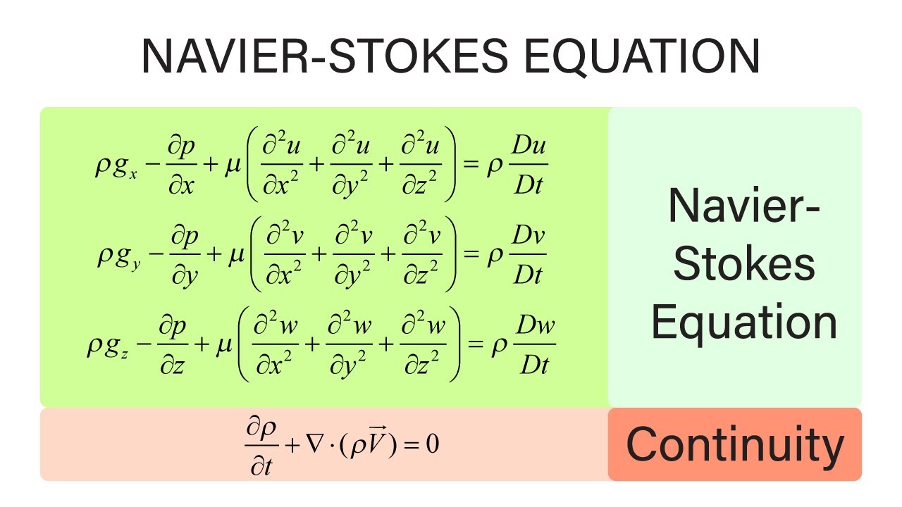
The formal development of the field of fluid dynamics started several centuries ago. Early physicists captured the continuum properties of fluid flow within a series of all-encompassing equations. These equations are known as the Navier-Stokes equations. However, there was a problem with these equations that signficantly stalled development of the study of fluids until only recently; they have no solution.

To understand this, consider how most equations (introduced outside of a gradulate level math course) are solved by defining the unknown variables as a function of the known quantities.

So, for example, 24 = 8 x Y can be rewritten as Y = 24 / 8 = 3. This is called an analytical solution.

However, when considering the broader mathematical environment, equations with an analytical solution an exception, and not the norm. There are many complex equations, partial differential equations in this case, that have no analytical solution.

For the Navier Stokes equations, the value at any point in the flowfield depends on the value at every point in the flowfield.

As a demonstration of the difficulty invovled with this, consider a sudoko puzzle. In any given cell, the value depends on every other value in the row & column it is within. For a 9x9 grid, it’s a 2-D dimensional puzzle with limited complexity that can be solved after some iteration.

Now consider the same puzzle, where instead of there just being a row and a column, there are thousands of connected dimensions.

There’s is beyond the purview of simple iteration.

Instead, approximate solutions have to be found with numerical methods. Numerical methods are a mathematically refined version of guess and check, and their use requires millions of arithmetic operations to slowly hone in on an approximate answer to an equations. Fortunately, computers are great at this.

Computational Power #

Moore’s Law observes that computational power has exponentially increased since the mass market adoption of the computer. This trend, combined with the availability of this power to the masses, is mirrored in the complexity of fluid simulations that are able to be solved through CFD.

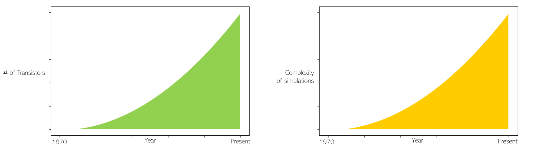
For example, the simulations used to develop the aerodynamics of the space shuttle, simulations run on the fastest supercomputers at the time, pale in comparison to the complexity of simulations that can be run on a desktop computer today.

Unfortunately, computers today still aren’t fast enough to solve the original Navier-Stokes equations. Even simulating airflow around a car would require more computing power than exists in the world combined. In fact, just storing the results from that simulation would not fit in all of the storage of the world. Such is the complexity of fluid dynamics.

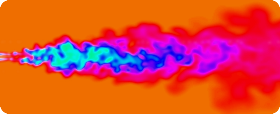
Turbulence #

To understand why, the concept of turblence needs to be reviewed. Simply put, turbulence is characterized by chaotic fluid flow. By contrast, laminar flows are smooth and orderly. Turblent flows are by and large the norm, as all fluid flows eventually become turbulent.

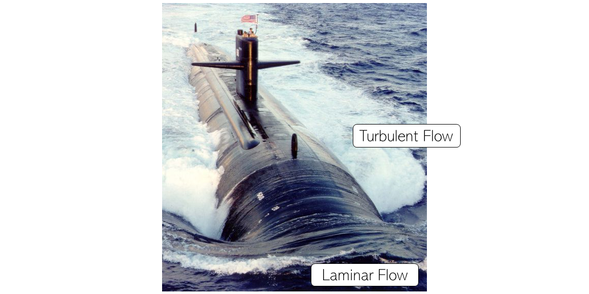
Laminar and Turbulent flow across a Los Angeles-class submarine. Photo courtesy of the US Navy.

Turbulent motion contains energy within it. Energy in turbulence starts off at the large visible scales, and eventually propogates to smaller and lower scales until it’s eventually converted to heat at the molecular level. This is termed the energy cascade.

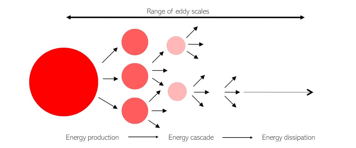
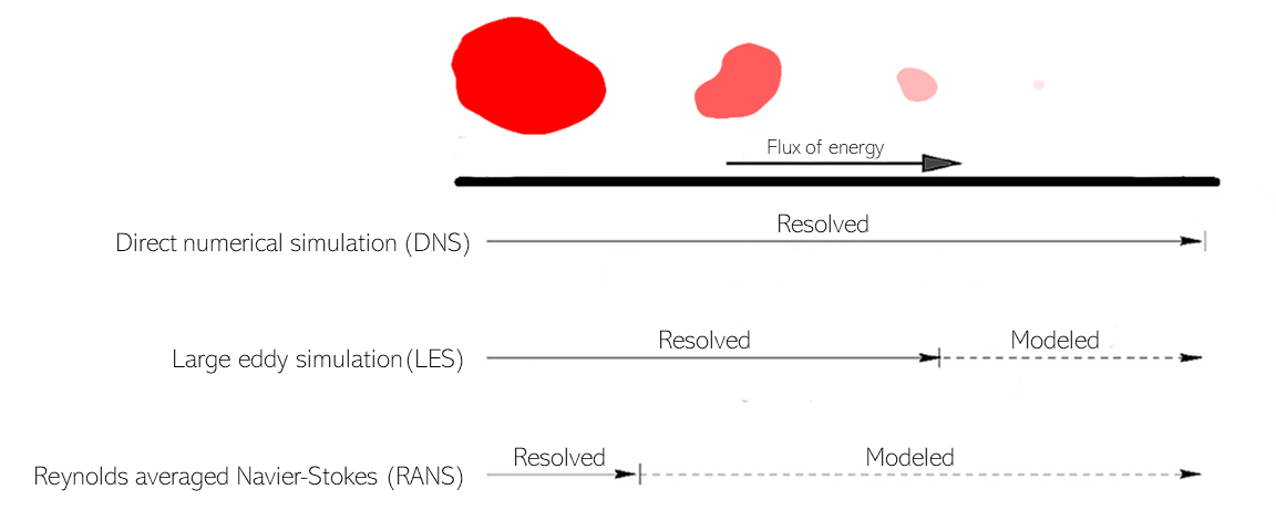
Direct numerical simulation (DNS) is a CFD methodology that resolves the physics of all the energy scales, from the largest down to the smallest. This makes it simultaneously the most accurate but computationally taxing simulation method. This is because some of the turblent length scales are on the order of particles. Ultimately, physicists and engineers are not willing to wait centuries for computers to evolve to a point where DNS CFD is practical, so alternatives have been developed.

Turbulence models are a way of resolving the largest scales of turbulence, which are typically the most important, while approximating the behavior of the smaller scales. This requires a small fraction of the book keeping without sacrificing too much accuracy.

It’s difficult to discuss turbulence modeling further without diving into highly technical material. For those interested, the series of articles titled Turbulence Modeling ForTheWin by Salient Edge do a good job at highlighting the development of such models, explained in the context of motorsport.

Richard Feynman
American Physics Nobel Prize Laureate Richard Feynman described turbulence as “the most important unsolved problem of classical physics”.

Transience #

Another fundamental complexity of fluid flow is its transient nature. To be transient means a phenomenon is variable with time. By contrast, steady state means to be constant with the passing of time.

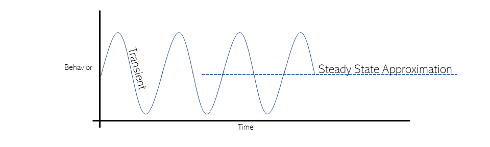
A steady state fluid dynamics problem is already very intricate, as there is 3D variation in complex flow quantities. Transient systems ramp up that complexity by adding a fourth dimension, as behavior changes in the spatial (3D) sense over time.

Steady state CFD fudges the fundamental equations to remove the time variability, reducing complexity by atleast an order of magnitude, but sacrificing accuracy along the way. Whether this is a worthwhile tradeoff is a case by case basis. It is often useful in the early stages of a project, when maximizing iterations takes precedence over maximizing accuracy. As a rule of thumb, ten steady state simulations can be run for the computational resources of 1 transient simulation. Eventually, steady state CFD becomes a large accuracy bottleneck.

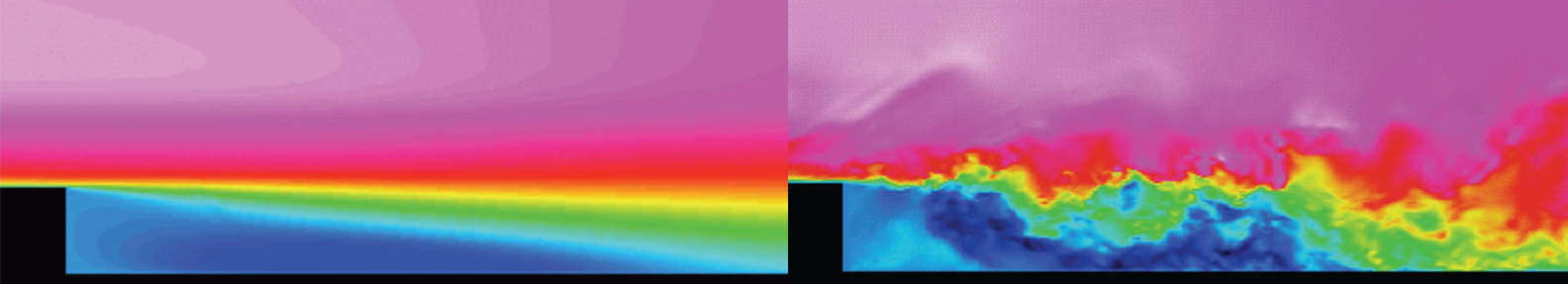
While steady state results are useful, one should be weary of drawing too many conclusions from them. For example, in the image below, the averaged flowfield is remarkably different to an image of the instantaneous transient flowfield.

Running CFD #

As discussed, CFD simply consists of a series of mathematical equations that are repeatedly solved to eventually hone in on an approximate solution. Fortunately, most commerical CFD packages heavily abstract the user from the mathematical underpinnings. The user makes a handful of high level decisions and the mathematics in the background are appropriately altered.

Boundary Conditions #

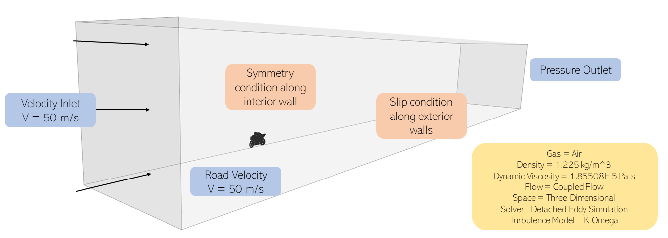
Running a simulation requires first defining the boundary conditions. These boundary conditions constrain the flow behavior to only what is desired.

For example, for an external aerodynamics case, the boundary conditions would be set up like the following:

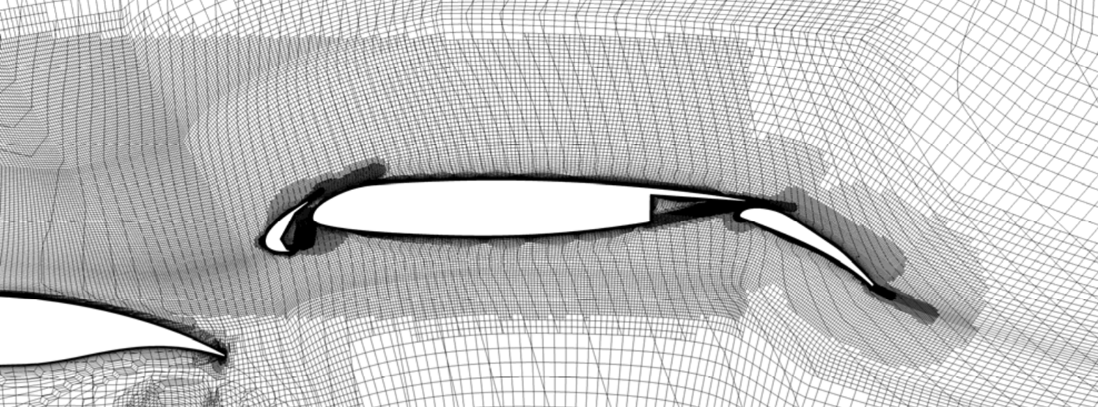
The Grid #

The governing equations are formulated to only describe simple, local fluid behavior. To use them to describe global flow phenmomenon, a CFD simulation takes a large, continuous domain and decomposes it into a grid. The equations describing fluid behavior are then iteratively solved in each cell. Areas where the physics are likely to be more complex are refined to better resolve the complexity.

The simulation initially starts off wildly inaccurate, as it’s little more than a guess in the early stages, but the longer simulation runs, it gets closer and closer to satifying the equations governing fluid flow.

Evenually, when the difference from one iteration to another is acceptably small, the simulation is considered done. The solution computes all of the flowfield data, resulting in an immense & complex dataset, analysis of which must be done in a granular fashion to obtain a qualitative understanding of the flowfield. See here for a discussion on how to effectively post process a CFD simulation.

Concluding Thoughts #

There is an old adage in engineering that all models are wrong, but some are useful. Truly remarkable engineering has and continues to be done with imperfect models.